
Excel Formulas List With Examples
Last updated on Jan 22, 2024

What is Excel?
Excel is a great tool for anyone who works with data. Whether you are a student or business owner or data analyst, it helps you to store, organize and analyze data. We can handle huge amounts of data in excel. You can store data in thousands of rows and columns, manipulate it and gain insights. Using excel we can also sort, filter and group data making it easy to identify patterns and trends. We can even share the excel sheets with others setting access permissions like, only view the data, edit, etc.
Excel has a number of applications in various sectors. It is used by individuals, businesses, organizations of all sizes for data analysis. You can create graphs, charts, reports and tables very easily. Using excel you can also perform calculations, automate the tasks and create your own formulas to solve complicated problems. So learning some of the basic excel formulas can help you master data analysis using excel. In excel we use several formulas to perform operations easily and effectively. Users can use these formulas to automate calculations, minimize errors, and obtain valuable insights from the data.
Want to gain knowledge in Excel? Then visit here to learn Excel Training !
Now let's go through the basic excel formulas list:
Basic Excel Formulas:
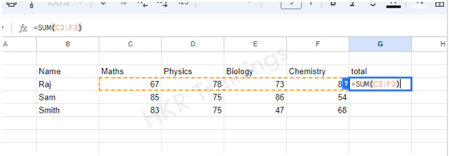
1. SUM
Purpose: It is used to add values in the cells.
Formula: If you want to add 4 cells in a row then you can write =SUM(C3:F3). You can also use this formula as an excel addition formula.
How to use the SUM formula in excel?
- First select a cell where you need the sum value
- Then type “=” sign
- Type SUM and open bracket "(" and select the range.
- Close the bracket ")" and hit the enter button
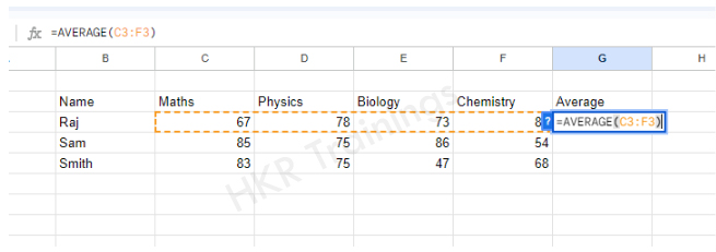
2. AVERAGE
Purpose: It is used to find the average of the values in the cells.
Formula: If you want to find the average of cells C3 to F3 then you can write =AVERAGE(C3:F3)
How to use the AVERAGE formula in excel?
- First select a cell where you need the AVERAGE value
- Then type “=” sign
- Type AVERAGE and open bracket “(” and select the range.
- Close the bracket “)” and hit the enter button
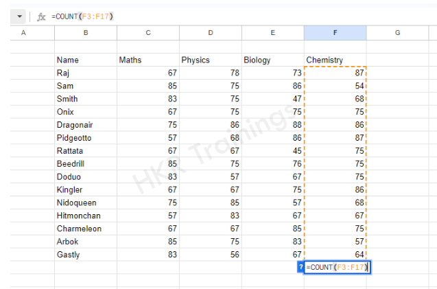
3.COUNT
Purpose: It is used to count the number of cells within the specified range of cells.
Formula: If you want to count the numbers in range F3 to F17 then you can write =COUNT(F3:F17)
How to use the COUNT function?
- First select a cell where you need the COUNT value
- Then type “=” sign
- Type COUNT and open bracket “(” and select the range.
- Close the bracket “)” and hit the enter button
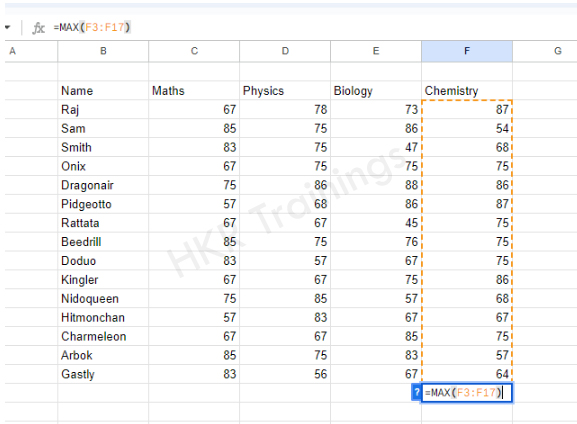
4. MAX
Purpose: It returns the maximum value from the specified range of cells.
Formula: If you want to find the maximum value in range F3 to F17 then you can write =MAX(F3:F17)
How to use the MAX function?
- First select a cell where you need the MAX value
- Then type “=” sign
- Type MAX and open bracket “(” and select the range.
- Close the bracket “)” and hit the enter button
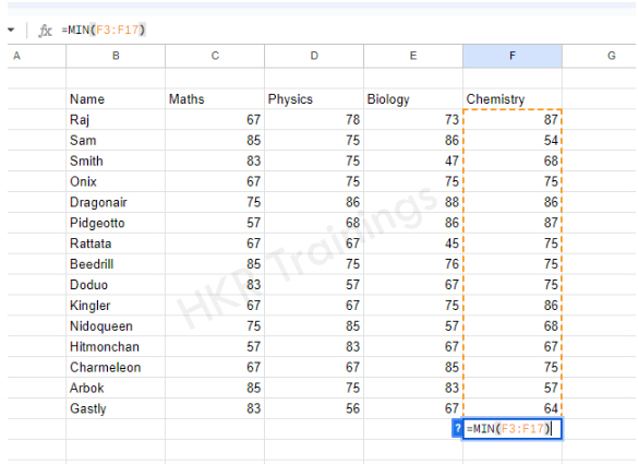
5. MIN
Purpose: It returns the minimum value from the specified range of cells.
Formula: If you want to find the minimum value in range F3 to F17 then you can write =MAX(F3:F17)
How to use the MIN function?
- First select a cell where you need the MIN value
- Then type “=” sign
- Type MIN and open bracket “(” and select the range.
- Close the bracket “)” and hit the enter button
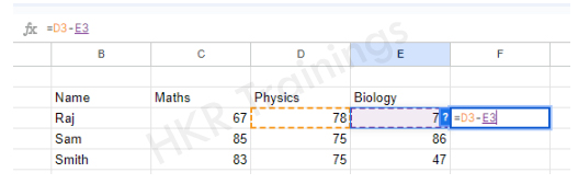
6.Subtraction
Purpose: It returns a difference of two specific cell values.
Formula: If you want to find the difference value of two cells D3 and E3 then you can write =D3-E3
How to use subtraction formula in Excel?
- First select a cell where you need the Subtracted value
- Then type “=” sign
- Select the cell from which you want the other value to be subtracted
- Then write “-” and select the other value that must be subtracted
- hit the enter button
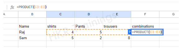
7. PRODUCT
Purpose: It multiplies two or more numbers .
Formula: If you want to multiply the values in the cells C3 to E3 then you can write =PRODUCT(C3:E3)
How to multiply in Excel?
- First select a cell where you need the PRODUCT value
- Then type “=” sign
- Type PRODUCT and open bracket “(” and select the range.
- Close the bracket “)” and hit the enter button
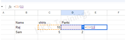
8. DIVIDE
Purpose: It is used to divide one number by another.
Formula: If you want to divide one value C3 by another value D3 then you can write =C3/D3. You can also use the same formula as the percentage formula in excel.
How to use the division formula in Excel?
- First select a cell where you need the result value
- Then type “=” sign
- Select the number that must be divided
- Then write forward slash “/” and select the other value that must divide the first number
- hit the enter button

Excel Training
- Master Your Craft
- Lifetime LMS & Faculty Access
- 24/7 online expert support
- Real-world & Project Based Learning
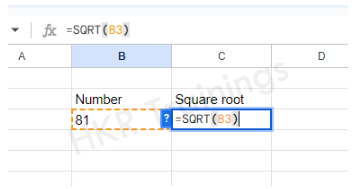
9. SQUARE ROOT
Purpose: It will calculate the square root of a number .
Formula: If you want to find the square root of a number B3 then you can write =SQRT(B3)
How to calculate square root in Excel?
- First select a cell where you need the Square root value
- Then type “=” sign
- Type SQRT and open bracket “(” and select the value you want to find square root.
- Close the bracket “)” and hit the enter button
Date and Time Formulas
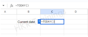
1. TODAY
Purpose: It will return the current date.
Formula: If you want to write the current date then you can write =TODAY(). We need not select any cell.
How to use the TODAY function in Excel?
- First select a cell where you want to write the date
- Then type “=” sign
- Type TODAY()
- Hit the enter button
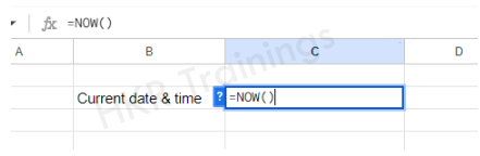
2. NOW
Purpose: It will return the current date and the time.
Formula: If you want to write the current date and time in a cell then you can write =NOW(). We need not select any cell.
How to use the NOW function in Excel?
- First select a cell where you want to write the date
- Then type “=” sign
- Type NOW()
- Hit the enter button
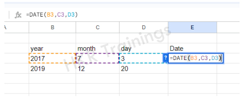
3. DATE
Purpose: Excel date formula will return a date based on the year, month and day specified.
Formula: If you want to write the date with a specific date D3, month C3, year B3, then you can write =DATE(B3,C3,D3). It supports year, month and day format.
How to use the DATE function in Excel?
- First select a cell where you want to write the date
- Then type “=” sign
- Type DATE and open bracket “(” and select the year and put a comma, select the month and put a comma and select the day
- Close the bracket “)” and hit the enter button
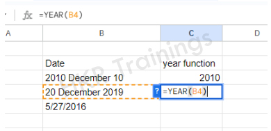
4. YEAR
Purpose: It will return the year from a date specified.
Formula: If you want to write only the year from a specified date (in the cell B4), then you can write =YEAR(B4).
How to use the YEAR function in Excel?
- First select a cell where you want to write the year
- Then type “=” sign
- Type YEAR and open bracket “(” and select the cell where you have written the date
- Close the bracket “)” and hit the enter button
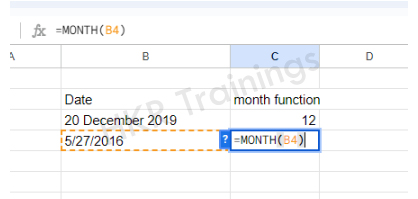
5. MONTH
Purpose: It will return the month from a date specified.
Formula: If you want to write only the month from a specified date (in the cell B4), then you can write =MONTH(B4).
How to use the MONTH function in Excel?
- First select a cell where you want to write the month
- Then type “=” sign
- Type MONTH and open bracket “(” and select the cell where you have written the date
- Close the bracket “)” and hit the enter button
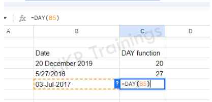
6. DAY
Purpose: It will return the day from a date specified.
Formula: If you want to write only the day of the month from a specified date (in the cell B5), then you can write =DAY(B5).
How to use the DAY function in Excel?
- First select a cell where you want to write the Day
- Then type “=” sign
- Type DAY and open bracket “(” and select the cell where you have written the date
- Close the bracket “)” and hit the enter button
Logical Formulas
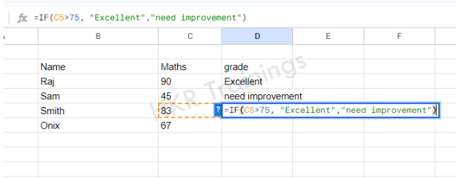
1. IF
Purpose: It is used to test a logical condition. If the condition is true it returns one value and if the condition is false it returns another value.
Formula: IF(condition, “value_if_condition_is_true”, “value_if_condition_is_false”)
How to use the IF condition in Excel?
- First select a cell where you want to write the result
- Then type “=” sign
- Type IF and open bracket “(” and write the condition and put a comma. Then write the value to be displayed if the condition is true in inverted commas and put a comma, and then write the value to be displayed if the condition is false in inverted commas.
- Close the bracket “)” and hit the enter button
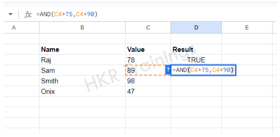
2. AND
Purpose: It is used to return true if the arguments(conditions) specified are true or else it returns false. AND will accept up to 225 arguments.
Formula: AND(condition_1, condition2, …… )
How to use AND function in Excel?
- First select a cell where you want to write the result
- Then type “=” sign
- Type AND and open bracket “(” and write the condition and put a comma. Then write another condition. You can write up to 225 conditions.
- Close the bracket “)” and hit the enter button
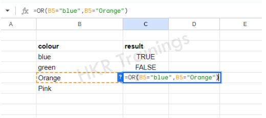
 3. OR
3. OR
Purpose: It is used to return true if any of the specified conditions is true or else it returns false. OR will accept up to 225 conditions.
Formula: OR(condition_1, condition2, …… )
How to use OR function in Excel?
- First select a cell where you want to write the result
- Then type “=” sign
- Type OR and open bracket “(” and write the condition and put a comma. Then write another condition. You can write any number of conditions up to 225 conditions.
- Close the bracket “)” and hit the enter button
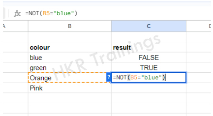
4. NOT
Purpose: It will return the opposite value of the condition. If the condition is true, NOT will return false. If the condition is false, NOT will return true.
Formula: NOT(condition)
How to use the NOT function in Excel?
- First select a cell where you want to write the result
- Then type “=” sign
- Type NOT and open bracket “(” and write the condition
- Close the bracket “)” and hit the enter button
Subscribe to our YouTube channel to get new updates..!
Text Formulas
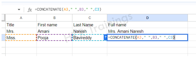
1. CONCATENATE
Purpose: Concatenate formula in excel will combine two or more text strings.
Formula: CONCATENATE(text1,text2,text3)
How to use the CONCATENATE function in Excel?
- First select a cell where you want to write the result
- Then type “=” sign
- Type CONCATENATE and open bracket “(” and select the cell which you want to display first, put a comma, select the other cell you wanted to display next, put a comma and select another cell you wanted to display next
- Close the bracket “)” and hit the enter button
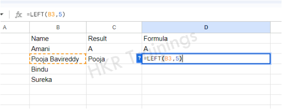
2. LEFT
Purpose: LEFT function will return the specified number of characters from the beginning of the text.
Formula: LEFT(cell, number_of_chars_to_display)
How to use the LEFT function in Excel?
- First select a cell where you want to write the result
- Then type “=” sign
- Type LEFT and open bracket “(” and select the cell from which you want to display the character, put a comma and write the number of characters to display
- Close the bracket “)” and hit the enter button
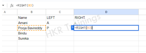
3. RIGHT
Purpose: RIGHT function will return the specified number of characters from the ending of the text.
Formula: RIGHT(cell, number_of_chars_to_display)
How to use the RIGHT function in Excel?
- First select a cell where you want to write the result
- Then type “=” sign
- Type RIGHT and open bracket “(” and select the cell from which you want to display the character, put a comma and write the number of characters to display
- Close the bracket “)” and hit the enter button
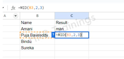
4. MID
Purpose: MID function will return the specified number of characters from the middle of the text, starting from the specified position.
Formula: MID(cell, starting_number, number_of_chars_to_display)
How to use the MID function in Excel?
- First select a cell where you want to write the result
- Then type “=” sign
- Type MID and open bracket “(” and select the cell from which you want to display the character, put a comma and write the starting number from where the character must be displayed, put a comma and write the number of characters to display
- Close the bracket “)” and hit the enter button
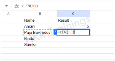
5. LEN
Purpose: LEN function will return the length of the text in number of characters.
Formula: LEN(select_the_cell_to_find_ length_of_text)
How to use the LEN function in Excel?
- First select a cell where you want to write the result
- Then type “=” sign
- Type LEN and open bracket “(” and select the cell to find the length of the text
- Close the bracket “)” and hit the enter button
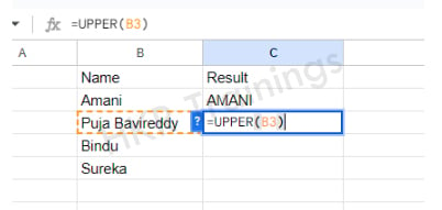
6. UPPER
Purpose: UPPER function will convert all the characters in the text to uppercase.
Formula: UPPER(select_the_text)
How to use the UPPER function in Excel?
- First select a cell where you want to write the result
- Then type “=” sign
- Type UPPER and open bracket “(” and select the cell to convert the characters to uppercase
- Close the bracket “)” and hit the enter button
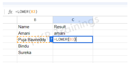
7. LOWER
Purpose: LOWER function will convert all the characters in the text to Lowercase.
Formula: LOWER(select_the_text)
How to use the LOWER function in Excel?
- First select a cell where you want to write the result
- Then type “=” sign
- Type LOWER and open bracket “(” and select the cell to convert the characters to lowercase
- Close the bracket “)” and hit the enter button
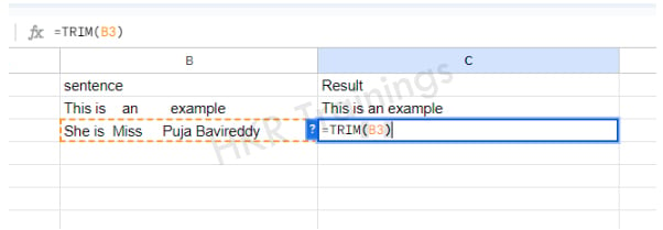
8. TRIM
Purpose: TRIM function will remove all the extra spaces from the text string.
Formula: TRIM(select_the_text)
How to use the TRIM function in Excel?
- First select a cell where you want to write the result
- Then type “=” sign
- Type TRIM and open bracket “(” and select the cell to remove all the extra spaces
- Close the bracket “)” and hit the enter button
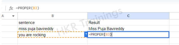
9. PROPER
Purpose: PROPER function will capitalize the first character of each word and converts the remaining characters to lower case.
Formula: PROPER(select_the_text)
How to use the PROPER function in Excel?
- First select a cell where you want to write the result
- Then type “=” sign
- Type PROPER and open bracket “(” and select the cell you wanted to make it proper
- Close the bracket “)” and hit the enter button
Top 30 frequently asked Excel Interview Questions !
Statistical formulas
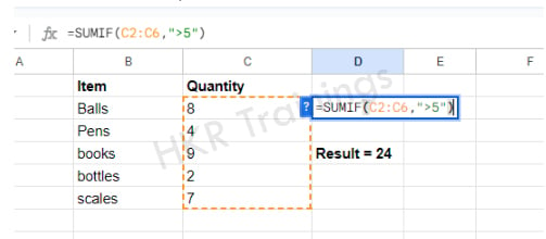
1. SUMIF
Purpose: SUMIF function will add all the values in a range of cells that satisfies a specific condition.
Formula: SUMIF(range, criteria, sum_range)
Here range is the range of the cell you want to evaluate, criteria is the condition you want to check and sum_range is the range of cells you wanted to add. If you skip the sum_range, the function will add the values in range.
How to use the SUMIF function in Excel?
- First select a cell where you want to write the result
- Then type “=” sign
- Type SUMIF and open bracket “(” and select the range, put a comma and write the criteria in inverted commas
- Close the bracket “)” and hit the enter button
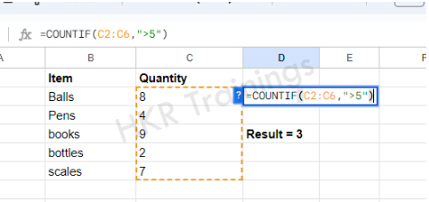
2. COUNTIF
Purpose: COUNTIF function in excel will count the number of cells in the range that satisfies a specific condition.
Formula: COUNTIF(range, criteria)
Here range is the range of the cell you want to evaluate and criteria is the condition you want to check.
How to use the COUNTIF formula in Excel?
- First select a cell where you want to write the result
- Then type “=” sign
- Type COUNTIF and open bracket “(” and select the range, put a comma and write the criteria in inverted commas
- Close the bracket “)” and hit the enter button
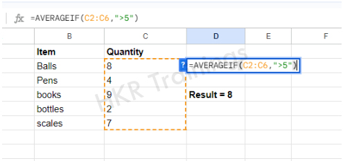
3. AVERAGEIF
Purpose: AVERAGEIF function will calculate the arithmetic mean of the values in the range of cells that satisfies a specific condition.
Formula: AVERAGEIF(range, criteria, average_range)
Here range is the range of the cell you want to evaluate, criteria is the condition you want to check and average_range is the range of cells you want to calculate the mean. If you skip the average_range, the function will calculate the mean of the values in range.
How to use the AVERAGEIF function in Excel?
- First select a cell where you want to write the result
- Then type “=” sign
- Type AVERAGEIF and open bracket “(” and select the range, put a comma and write the criteria in inverted commas
- Close the bracket “)” and hit the enter button
Lookup and Reference formulas
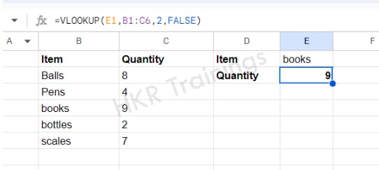
1. VLOOKUP
Purpose: VLOOKUP function will search for a particular value in the first column of the table or range and returns a corresponding value from a particular column in the same row.
Formula: VLOOKUP(lookup_value, table array, column_index_number, range_lookup)
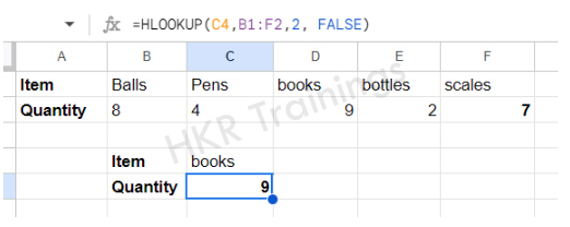
2. HLOOKUP
Purpose: HLOOKUP function will search for a particular value in the first row of the table or range and returns a corresponding value from a particular column in the same column.
Formula: HLOOKUP(lookup_value, table array, row_index_number, range_lookup)
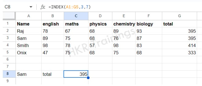
3. INDEX
Purpose: INDEX function will return the value of a cell in a specified row and column within a range or table
Formula: INDEX(cells_range, row_number, col_number)
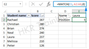
4. MATCH
Purpose: MATCH function will search for a particular value within a range of cells and will return a relative position of the value within the range
Formula: MATCH(lookup_value, cells_range, match_type)
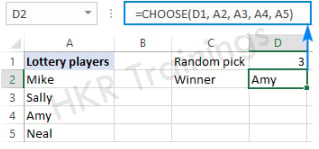
5. CHOOSE
Purpose: CHOOSE function will return a value from the values list according to the specified index number.
Formula: CHOOSE(index_num, value1, value2,....)
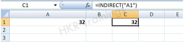
6. INDIRECT
Purpose: INDIRECT function will return a value from the values list according to the specified text string that contains a cell reference.
Formula: INDIRECT(reference_text, A1)
Financial formulas
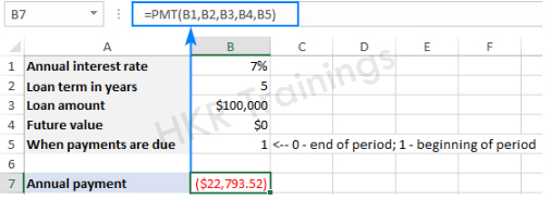
1. PMT
Purpose: PMT function will calculate the periodic payment for a loan or investment according to a fixed interest rate, term and loan amount.
Formula: PMT(rate, nper, pv, [fv], [type])
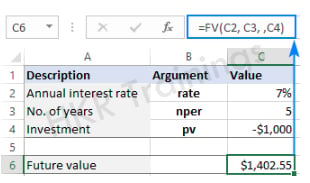
2. FV
Purpose: FV function will calculate the future value of the investment according to a fixed interest rate, term and initial investment amount.
Formula: FV(rate, nper, pmt, [pv], [type])
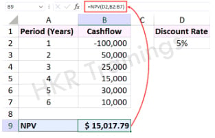
3. NPV
Purpose: NPV function will calculate the net present value of a series of cash flows according to a specified discount rate
Formula: NPV(rate, value1, value2, ….)
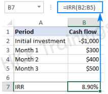
4. IRR
Purpose: IRR function will be the internal rate of return for a series of cash flows.
Formula: IRR(values, [guess])
Conclusion:
In this article we have discussed the basic excel formulas and their purpose with examples. We hope you found this article informative. For more articles stay tuned.
Related Articles:
About Author
Upcoming Excel Training Online classes
| Batch starts on 23rd Jul 2026 |
|
||
| Batch starts on 27th Jul 2026 |
|
||
| Batch starts on 31st Jul 2026 |
|
FAQ's
.